
5 Steps to Calculate DCF for Growth Stocks
Learn the essential steps to calculate DCF for growth stocks, ensuring accurate valuations through cash flow projections and sensitivity analysis.

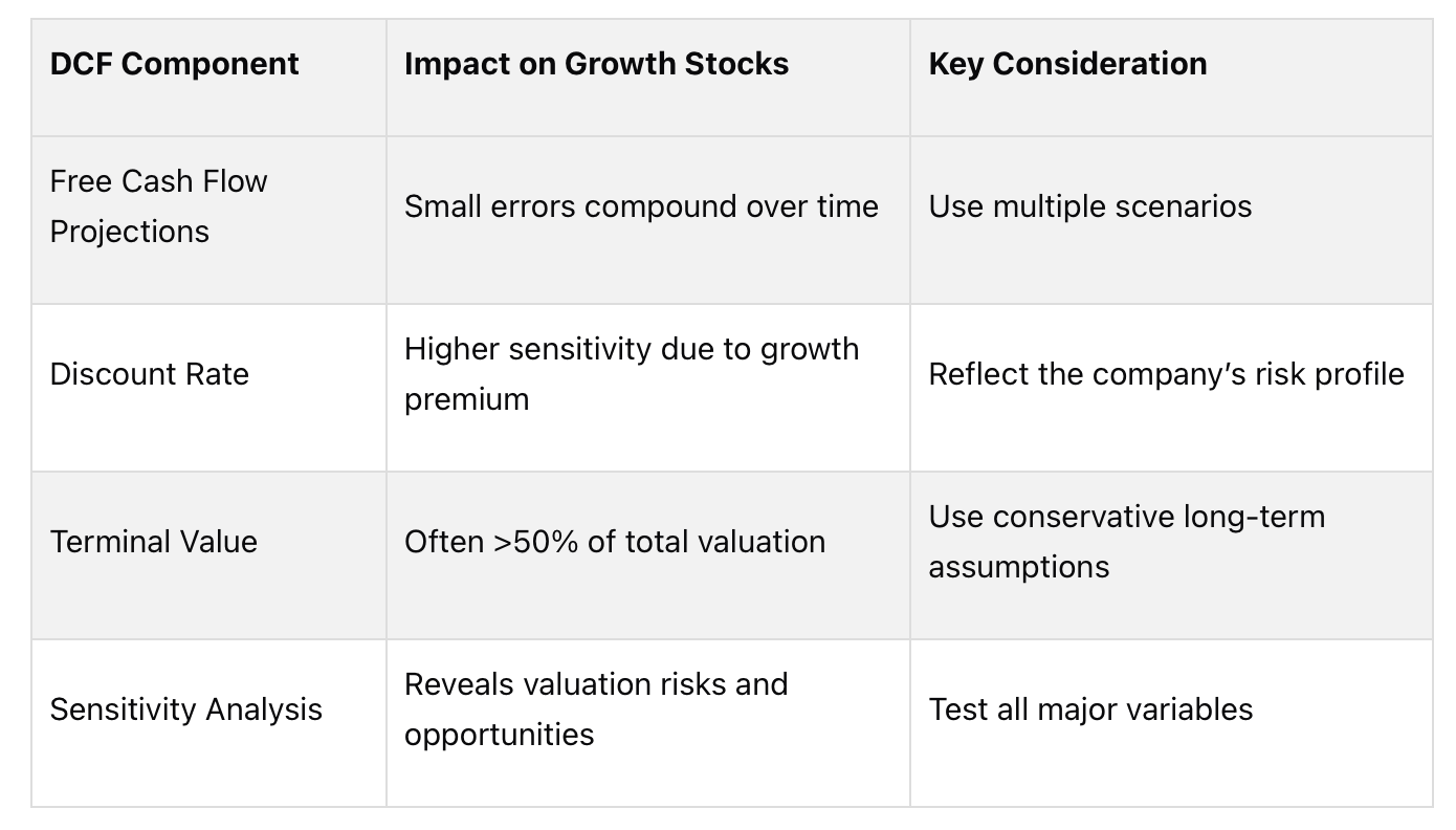
Discounted Cash Flow (DCF) is a go-to method for estimating a company’s intrinsic value, especially for growth stocks. It forecasts future free cash flows (FCF) and discounts them back to their present value using a discount rate. Here’s the process in simple steps:
Project Free Cash Flows (FCF): Forecast the company’s FCF for 5–10 years based on revenue growth, expenses, and capital expenditures.
Calculate the Discount Rate: Use the Weighted Average Cost of Capital (WACC) or Cost of Equity to reflect the investment’s risk and time value of money.
Estimate Terminal Value: Choose between the Gordon Growth Model or Exit Multiple Method to value cash flows beyond the forecast period.
Discount Cash Flows: Convert future cash flows and terminal value into present value using the discount rate.
Test Assumptions: Run sensitivity analyses to understand how changes in key variables (growth rate, discount rate, etc.) impact the valuation.
For growth stocks, terminal value often makes up 50–70% of the total valuation, and even small changes in assumptions can significantly impact results. Use conservative estimates and test multiple scenarios to ensure accuracy. By following these steps, you can determine whether a stock is undervalued or overvalued relative to its market price.
Build a Discounted Cash Flow (DCF) Model in Excel | Step-by-Step Valuation Guide
Step 1: Project Free Cash Flows
Start by forecasting a growth stock’s free cash flows (FCF) over the next 5–10 years - this is the foundation of your discounted cash flow (DCF) analysis. FCF represents the cash a company generates after covering its operating expenses and capital expenditures. This cash can either be distributed to shareholders or reinvested to fuel further growth.
The projection period typically spans 5–10 years, depending on the company’s growth stage, industry standards, and how predictable its future cash flows are. If a company is expected to maintain high growth for an extended time, you might opt for a longer forecast. However, the further into the future you go, the harder it becomes to make accurate predictions. To get started, break down revenue and expenses to create a clear and detailed cash flow projection.
Build Revenue and Expense Projections
To create reliable revenue and expense projections, lean on a mix of historical financial data, industry reports, management insights, and current market trends. Begin by examining the company’s revenue growth over the past three to five years. Look for patterns, seasonal fluctuations, and any one-off events that may have influenced results. For instance, a tech company with 20% annual growth in recent years might see that rate slow to 15% if market saturation is approaching - or even accelerate if new products or innovations are on the horizon.
Operating expenses and capital expenditures (CapEx) can be forecast using historical ratios, planned investments, and industry benchmarks. Growth companies often benefit from economies of scale, where expenses grow at a slower rate than revenue. For example, a SaaS business might see CapEx decline as it scales, while a manufacturing company may need consistent investment in equipment and facilities.
Here’s a practical example: A U.S.-based software company generated $100 million in revenue last year, with a historical growth rate of 20%. For a baseline projection, you might assume 15% annual revenue growth, a 25% operating margin, and CapEx at 10% of revenue. In Year 1, this would result in:
Revenue: $115 million
Operating Income: $28.75 million (25% of revenue)
CapEx: $11.5 million (10% of revenue)
Free Cash Flow: $17.25 million
Repeat this calculation for each subsequent year, adjusting assumptions as the company matures.
Once you’ve established a solid baseline, explore alternative growth scenarios to account for uncertainty.
Create Multiple Growth Scenarios
Given the uncertainties in forecasting growth stocks, it’s essential to create multiple scenarios - conservative, base, and aggressive - that reflect a range of possible outcomes:
Conservative Scenario: Assumes slower revenue growth, tighter margins, and higher expenses due to factors like economic challenges or increased competition.
Base Scenario: Represents the most likely outcome, typically aligned with historical performance and adjusted for current market conditions.
Aggressive Scenario: Envisions faster growth, driven by rapid market adoption, successful product launches, or early entry into new markets - while staying grounded in realistic assumptions.
Here’s how these scenarios might compare:

For example, a conservative case might assume 10% annual revenue growth with 20% operating margins, while an aggressive case could project 25% growth with expanding margins due to operational efficiencies. Clearly documenting these assumptions is crucial, especially for sensitivity analyses or when presenting your valuation to stakeholders.
Growth companies, particularly those operating at the forefront of market shifts or technological advancements, can be tricky to forecast.
Step 2: Calculate the Discount Rate
The discount rate represents the return investors expect for taking on the risks associated with a particular investment. Essentially, it’s the minimum return needed to make a growth stock more appealing than a safer alternative like U.S. Treasury bonds. Even small changes in this rate can have a big impact on a stock’s valuation. It’s a key element in Discounted Cash Flow (DCF) analysis, as it accounts for both the time value of money and the risks tied to future cash flows.
The time value of money recognizes that a dollar today holds more value than a dollar received in the future. On top of that, the discount rate includes a risk premium to account for uncertainties in cash flows. Growth stocks, with their unpredictable earnings, often carry a higher risk premium.
Factors That Influence Discount Rates
Several factors come into play when determining the discount rate for growth stocks:
Market risk: Factors like interest rate fluctuations, economic downturns, and market volatility can drive discount rates higher. For example, rising interest rates or heightened economic uncertainty often lead to increased discount rates.
Company-specific risk: Growth stocks face unique challenges, such as unproven business models, reliance on key personnel, competitive pressures, or regulatory hurdles. A biotech company awaiting FDA approval has a very different risk profile compared to a mature software firm with steady subscription income. Higher risks demand higher discount rates.
Investor expectations: Investors in growth stocks usually accept higher risks in exchange for the potential of greater returns. If similar companies in the sector are delivering annual returns of 15–20%, the discount rate should reflect these expectations. Optimistic markets tend to lower required returns, while bearish markets push them higher.
For U.S. growth stocks, discount rates typically range from 8% to over 20%, depending on the company’s risk profile and the broader market environment. A stable tech giant may justify a lower rate, while a fledgling electric vehicle startup could require an 18% or higher rate to account for its higher risks and uncertainties.
WACC vs. Cost of Equity
Once the factors influencing the discount rate are clear, the next step is choosing the right method for calculating it. This decision depends heavily on the company’s capital structure - whether it’s primarily financed through debt, equity, or a mix of both.
Weighted Average Cost of Capital (WACC): This method blends the cost of debt and equity, making it more suitable for companies with significant debt in their capital structure. If debt accounts for 25% or more of the company’s financing, WACC provides a more accurate picture of the overall cost of capital.
Cost of Equity: For growth companies that rely mostly on equity financing - often with little to no debt - this method is more appropriate. When debt makes up less than 10–15% of the capital structure, using the cost of equity simplifies the analysis without losing precision.
Let’s break it down with an example. Consider a U.S. tech growth stock with minimal debt. Assume the 10-year U.S. Treasury yield (risk-free rate) is 4.5%, the market risk premium is 5.5%, and the company’s beta is 1.8, meaning it’s 80% more volatile than the overall market. Using the Capital Asset Pricing Model (CAPM):
Cost of Equity = 4.5% + (1.8 × 5.5%) = 14.4%
This 14.4% would serve as the discount rate for the DCF analysis.
As market conditions evolve, the discount rate should be adjusted. For instance, rising interest rates increase the risk-free rate, while economic uncertainty can push up the market risk premium. During the 2022 interest rate hikes, many growth stock discount rates climbed from 10–12% to 15–18% or higher, reflecting both higher base rates and greater uncertainty about future growth.
Companies operating in emerging or rapidly changing markets face unique valuation challenges. In these cases, traditional discount rate models may need to be adjusted to better capture the specific risks and rewards. Tools like Trending Tickers can help investors identify opportunities where broad market trends and individual innovation come together, offering insights into how to fine-tune discount rates for such scenarios.
Step 3: Estimate Terminal Value
Terminal value often represents a significant portion - typically 50–70% - of a growth stock’s discounted cash flow (DCF) valuation. It accounts for all cash flows beyond the forecast period. In essence, terminal value reflects the long-term value of a company. For instance, if you’re forecasting a tech company’s cash flows through 2030, the terminal value captures everything from 2031 onward.
Choose a Terminal Value Method
There are two main approaches to calculating terminal value: the Gordon Growth Model and the Exit Multiple Method.
The Gordon Growth Model assumes that cash flows will grow at a constant, perpetual rate after the forecast period. The formula is as follows:
Terminal Value = FCF(n+1) / (r - g)
Here:
FCF(n+1) is the free cash flow in the first year after the forecast period.
r is the discount rate.
g is the perpetual growth rate.
For example, imagine a software company with a projected free cash flow of $50 million in the terminal year, a discount rate of 10%, and a perpetual growth rate of 3%:
$50,000,000 / (0.10 - 0.03) = $714,285,714.
The Exit Multiple Method, on the other hand, applies a valuation multiple - based on market data - to a financial metric from the final forecast year. For example, if comparable companies are trading at 15x EBITDA and your company projects $60 million in terminal year EBITDA:
15 × $60,000,000 = $900,000,000.
Here’s a quick comparison of the two methods:

The Gordon Growth Model is often a better fit for companies expected to stabilize into steady cash flow generation, such as a high-growth SaaS company that eventually matures into predictable subscription revenues. The Exit Multiple Method works well when reliable comparable company data is available, particularly in industries like retail or manufacturing, where valuation benchmarks are well-established.
Once you’ve chosen a method, the next step is to define realistic long-term growth assumptions to finalize your terminal value estimate.
Establish Long-Term Growth Assumptions
When using the Gordon Growth Model, perpetual growth rates for U.S. companies typically fall between 2–3% annually. These rates align with expected inflation and GDP growth. Setting a growth rate higher than this range can imply that the company will eventually outpace the broader economy - an unlikely scenario.
For example, a dominant platform company might justify a rate closer to 3%, reflecting its ability to grow alongside the digital economy. Meanwhile, a cyclical growth company might need a more cautious assumption, around 2–2.5%.
If you’re opting for the Exit Multiple Method, selecting the right multiple requires analyzing comparable companies with similar size, profitability, growth potential, and risk profiles. Common valuation multiples for U.S. growth stocks include EV/EBITDA for profitable companies and EV/Revenue for those still scaling. For instance:
A high-growth cloud software company might trade at 8–12x revenue.
A mature tech company could trade at 15–25x EBITDA.
It’s crucial to stress-test your inputs, as terminal value has an outsized impact on the overall valuation. Running sensitivity analyses - adjusting key variables within a reasonable range - can help you understand how dependent your valuation is on these assumptions.
Finally, consider market conditions when choosing a method. During volatile periods, the Exit Multiple Method may be less reliable due to fluctuating market multiples. In contrast, the Gordon Growth Model can provide more stability if you’re confident in your long-term growth projections.
Step 4: Discount Cash Flows to Present Value
To account for the time value of money - factoring in opportunity costs and risks - forecasted cash flows and terminal value must be converted into present value. This step is particularly crucial for growth stocks, where a significant portion of their value depends on cash flows far into the future.
Calculate Discount Factors and Discount Cash Flows
The Discounted Cash Flow (DCF) formula can be broken into a series of steps. The first step is to calculate the discount factor for each year using the formula:
Discount Factor = 1 ÷ (1 + r)^n
Here, r represents the discount rate, and n is the year number.
Let’s break it down with an example. Imagine a cloud software company projecting free cash flows of $15 million, $22 million, and $30 million for the next three years, with a terminal value of $180 million. Assuming a discount rate of 12%:
Year 1: $15,000,000 × 0.893 = $13,395,000
Year 2: $22,000,000 × 0.797 = $17,534,000
Year 3: $30,000,000 × 0.712 = $21,360,000
Terminal Value: $180,000,000 × 0.712 = $128,160,000
Notice how the discount factors decrease over time, which reflects how future cash flows lose value as they are pushed further into the future. The terminal value gets the same discount factor as Year 3 because it represents the value at the end of the forecast period.
By applying these discount factors, you standardize all future cash flows into present value terms. The 12% discount rate in this example represents the company’s cost of capital, accounting for both investment risks and other opportunities available to investors. This step sets the stage for calculating the enterprise value.
Calculate Total Stock Value
Once the cash flows are discounted, the next step is to sum them up to determine the enterprise value, which represents the total value of the business. Using the example above:
$13,395,000 + $17,534,000 + $21,360,000 + $128,160,000 = $180,449,000
To calculate the equity value per share, follow two additional steps. First, subtract any net debt from the enterprise value. If the company has $5 million in net debt, the equity value becomes $175,449,000. Second, divide this figure by the number of shares outstanding. For 10 million shares, each share would be worth approximately $17.54.
This per-share value provides an estimate of the stock’s intrinsic worth based on its ability to generate future cash flows. Comparing this value with the current market price helps determine if the stock is undervalued or overvalued.
The strength of this method lies in its clarity. Every assumption - whether it’s growth rates or discount rates - directly influences the final valuation. However, this also means that small changes in these inputs can lead to significant shifts in the results. That’s why the next step involves stress-testing these assumptions using sensitivity analysis.
It’s worth noting that terminal value often has the largest impact on the overall valuation. In this example, the terminal value accounted for more than 70% of the enterprise value.
Step 5: Test Your Assumptions
The DCF valuation you’ve calculated is only as good as the assumptions it’s built on. Even small tweaks to growth rates, discount rates, or terminal value assumptions can significantly impact your estimate. That’s why it’s crucial to test these variables and understand their influence on your valuation. This step takes your cash flow projections further by quantifying how sensitive they are to key factors.
Stress-Test Key Variables
Once you’ve calculated cash flows and discounted them, it’s time to take a closer look at the assumptions driving your numbers. Focus on stress-testing major variables like revenue growth, the discount rate, operating margins, and terminal value. These elements are critical in determining present value, and they’re often the most unpredictable - especially for high-growth companies.
Start by adjusting each variable one at a time. For example, if your base case assumes 25% annual revenue growth, test scenarios with growth rates of 23% and 27%. This gives you a sense of how changes in growth projections might affect your valuation.
The discount rate is another key factor that directly influences every cash flow in your model. Try varying it by 0.5–1%. A small shift in the discount rate can have a big impact - potentially altering the calculated per-share value by 10–15%.
Terminal value assumptions deserve extra attention since they often make up a large chunk of a growth stock’s total value. Test different terminal growth rates, such as 3%, 4%, and 5%, or experiment with alternative methods like exit multiples instead of perpetual growth rates.
Operating margin assumptions are also worth testing, particularly for companies still working toward profitability. Explore scenarios where margins improve faster or slower than expected to see how competitive pressures or cost changes could affect your valuation.
Display Sensitivity Analysis Results
Once you’ve tested these variables, it’s helpful to visualize the results to pinpoint which ones have the most significant impact. Sensitivity tables are a great way to do this. For instance, here’s an example of how equity value per share might change based on different combinations of discount rates and terminal growth rates:

This table highlights how much a stock’s intrinsic value can fluctuate based on your assumptions, emphasizing the importance of thorough stress-testing.
Other tools, like tornado diagrams, can help rank variables by their impact on valuation. For instance, you might find that changes in terminal growth rates have a much larger effect than adjustments to revenue growth rates. This can guide you to focus your research on the most influential assumptions.
Line graphs are another option. Plotting valuation outcomes against a single variable - like discount rates ranging from 8% to 16% - can reveal whether your model is particularly sensitive to changes in the cost of capital.
The goal here isn’t to predict one exact valuation but to understand a range of possible outcomes and identify which assumptions carry the most weight. This insight helps you evaluate whether a stock’s market price provides enough margin of safety given the uncertainties in your projections.
As market conditions evolve or new information about a company becomes available, you can revisit your sensitivity analysis. This makes your DCF model a living tool for ongoing investment decisions, rather than a static, one-time calculation.
Final Thoughts on DCF for Growth Stocks
Building on the steps we’ve covered, it’s clear that DCF remains a powerful tool for evaluating growth stocks. At its core, DCF focuses on a company’s ability to generate future cash flows, making it an essential part of any investor’s toolkit.
Key Points for Investors
The DCF process involves several critical steps: projecting cash flows, selecting a discount rate, estimating terminal value, discounting those values, and conducting sensitivity analysis. Each of these steps plays a significant role in shaping the final valuation, and even small adjustments can have a big impact.
For growth stocks, terminal value often accounts for 50–70% or more of the total valuation. Using conservative estimates here can help avoid overpaying for companies that might not meet their full potential.
The discount rate is another crucial factor. It should reflect the company’s risk profile accurately. A slight tweak to the discount rate can lead to large swings in valuation, so researching comparable companies and industry benchmarks is essential.
Sensitivity analysis is particularly important for growth stocks, as they tend to be more unpredictable. By stress-testing variables like revenue growth, operating margins, and terminal value assumptions, you can identify which factors have the most influence on your valuation and where the biggest risks lie.
Next Steps for Using DCF
Now it’s time to put this framework into action. Start applying DCF to the growth stocks you’re analyzing. Gather reliable data, create projections, and work through each step methodically. DCF analysis requires discipline and should be updated regularly.
It’s also a good idea to use other valuation methods alongside DCF. Techniques like comparable company analysis or precedent transactions can serve as useful checks, especially if your DCF results seem overly optimistic or overly cautious.
Stay up-to-date with macroeconomic trends and industry shifts that could influence your assumptions. Tools like Trending Tickers can help highlight growth stocks with strong fundamentals and favorable market conditions before they gain widespread attention. Combining market insights with a solid DCF approach puts you in a better position to act before trends become mainstream.
Keep in mind that DCF isn’t a “set-it-and-forget-it” exercise. As new financial data emerges or market conditions change, your model should evolve too. Regular updates ensure your analysis stays relevant and accurate.
The goal isn’t to predict the future perfectly - it’s to make informed decisions based on reasonable assumptions and to understand the range of possible outcomes. When you pair a well-executed DCF analysis with ongoing market research, you set yourself up for smarter, long-term investments in growth stocks.
FAQs
How do I choose the right discount rate for a DCF analysis of a growth stock?
To figure out the right discount rate for your DCF (Discounted Cash Flow) analysis of a growth stock, the go-to method is typically using the company’s weighted average cost of capital (WACC). This metric represents the average return investors expect, factoring in both equity and debt financing.
When dealing with growth stocks, you might need to tweak the rate to reflect the higher risk involved. Start by estimating the company’s cost of equity - often calculated using models like the Capital Asset Pricing Model (CAPM) - and its cost of debt. From there, determine the WACC by combining these components according to the company’s capital structure. Since growth stocks often come with more uncertainty, it’s reasonable to use a slightly higher discount rate to account for this added risk.
How do the Gordon Growth Model and Exit Multiple Method differ when estimating terminal value?
The Gordon Growth Model and the Exit Multiple Method are two widely used techniques for estimating terminal value in a discounted cash flow (DCF) analysis. While both serve the same purpose, they rely on different assumptions and calculations.
The Gordon Growth Model is based on the idea that cash flows will grow at a constant rate indefinitely. This makes it a great fit for businesses with stable and predictable growth patterns. The formula for this method is:
Terminal Value = Final Year Cash Flow × (1 + Growth Rate) / (Discount Rate − Growth Rate).
On the flip side, the Exit Multiple Method determines terminal value by applying a valuation multiple (like EV/EBITDA or P/E ratio) derived from comparable companies. This approach is often preferred for businesses with uncertain growth or when market-based metrics are more relevant.
The choice between these methods depends on the specific characteristics of the company and the data available. For companies with steady, mature growth, the Gordon Growth Model is typically more suitable. However, for growth stocks or businesses with fluctuating performance, the Exit Multiple Method often provides a more grounded estimate.
How can sensitivity analysis improve DCF valuation for growth stocks, and which key factors should I consider?
Sensitivity analysis adds depth to DCF valuation by illustrating how shifts in key assumptions can influence a stock’s value. It allows investors to pinpoint the most impactful variables, offering a clearer view of potential risks and outcomes.
Key areas to examine during sensitivity analysis include the discount rate, cash flow growth rate, and terminal value assumptions. By tweaking these factors, you can explore various scenarios, fine-tune your valuation, and make more confident investment decisions.